Covariance Matrix with Monte-Carlo simulations
What does the Matrix look like?
Caracteristics of the data: (see also MC Diagonal)
Data simulated @ CC
| group/runname | simupapier6 |
| bolo | 143-5 |
| nSide | 512 |
| IMO | '1127593' |
| signal name | 'cmb_gal_dipcosmo_gauss' |
| first ring | 580 |
| last ring | 13080 |
| Noise | White Noise (WN) sigma=62e-6 |
Commentary:
- simupapier6 corresponds to the new PPL (with the long ring) and in LSCmission mode_phase_pointing="random" (not "ideal")
date:04/06/09
The matrixes hereafter were obtained with 7600 MC simulations.
CONCLUSION:
- One can easily see the 1-year-delayed under-diagonal and the 6-month-delayed under-diagonal is clear on the Averaged MC matrix.
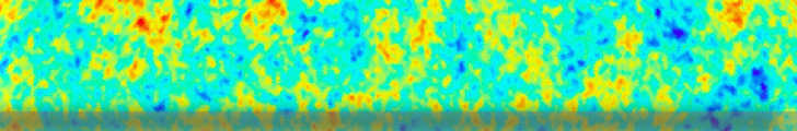
Matrix Display:
| MC Covariance Matrix low-resoluted with OP method | MC Covariance Matrix low-resoluted with Avg method | Polka Cov matrix |
 |  |  |
date:25/05/09
The matrix hereafter was obtained with 2000 MC simulations.
CONCLUSION:
- One can easily see the diagonal of the covariance matrix of offsets. (for more information on the diagonal see MC Diagonal).
- The average level (~1e-13) is consistent with the level of the noise used for the simulation (see also MC Diagonal).
- The 1-year-delayed under-diagonal is merely observable with 2000 MC simus. More simulations are required to see it clearly. Nevertheless, it is visible thanks to histograms around the antidiagonal (see MC AntiDiagonal)).
Matrix Display: