1.  Cross covariance limit cases

For cross qml, the covariance read Cov(C_\ell,C_{\ell'}) = \frac12 (F^{-1} G F^{-1} + F^{-1}) . We compare the diagonal of those two terms depending on the noise level :

1 muK	5 muK	50 muK	100 muK	500 muK

2.  MC vs TH mode-mode covariance matrix :

• nisde = 4
• nsimu = 1000
• For each figure :
  • First case (0,0) is the diagonal of the covariance matrix
  • Each following line correspond to a mode
  • First column correspond to EE , the second to BB

muK	mode	log scaled matrices theoretical (left) VS Monte-Carlo (right)
0.1
1.0
10
50

3.  Xpol Variance tests :

3.1  Nisde=32, plotting ratio of variance for EE then BB.

fsky	0.8	0.6	0.5	0.4

• For BB : we recover the xmql results between the ratio : ratio(at low noise) = fsky*ratio(at high noise). This means that the variance goes as 1/fsky for low noise, and 1/fsky^2 for high noise.

3.2  Nside = 128 and 256

fsky	0.8	0.6	0.5	0.4
			Attach:xpol2_Ns128.png Δ

fsky	0.7	0.5

• We observe oscillations for low noise level in BB. Those are actually linked to the signal of EE (see next figure for comparison). When the EE signal is low, leakage is low, and the variance ratio of BB between full and cut sky is

4.  New tests :

Comparaison effet de fsky et de masque :

• fsky = 1.0 VS fsky=0.5
• 3 types de masques : polar cap, litebird (=planck dust map), et random.
• nside=4
• nsimu = 1000
• beam =0.5 deg
• delta ell = 1 (non binning)
• r=0.1
• Cross and auto results are similar, thus only cross results are shown.
• Correlation matrices are computed as \displaystyle Corr = \frac{F^{-1}_{ij}}{\sqrt{F^{-1}_{ii} F^{-1}_{jj}}} where F is the fisher matrix.
• Global variance is computed as follow : \Delta_\alpha = C_\ell^{th} C^{-1}_{\ell \ell'} C_{\ell'}^{th} with C^{-1}_{\ell \ell'} = F_{\ell \ell'} the inverse of the mode covariance, namely the fisher matrix.
• Global variance computed certain mode range : \Delta_\alpha^{fsky=0.5} / \Delta_\alpha^{fsky=1.0} , nside=4 for BB

noise level	Cl type	\ell= 7	8	9	10	11
Analytic muK = 0.1	classic	0.4636	0.4442	0.4242	0.4141	0.4253
MC muK = 0.1	classic	0.4774	0.4899	0.4552	0.4529	0.4582
Analytic muK = 10	classic	0.3824	0.3688	0.3598	0.3568	0.3577
MC muK = 10	classic	0.4011	0.4065	0.3728	0.364	0.3625
Analytic muK = 1	classic	0.4549	0.4345	0.4144	0.4014	0.4093
MC muK = 1	classic	0.4678	0.4829	0.4418	0.4381	0.4444
Analytic muK = 50	classic	0.2752	0.2812	0.2844	0.286	0.2871
MC muK = 50	classic	0.3069	0.3151	0.3161	0.3184	0.3184

4.1  Polar (BB)

• First plot : spectrum estimation
• Left matrice : Global variance from \ell_{min} to \ell_{max} .
• Right matrix : Correlation matrice

Cl

Cl classic

Masks
10
10
1
1
0.1
0.1

Cl flat = 1e-17

10
10
1
1
0.1
0.1

Cl null = 0

10
10
1
1
0.1
0.1

5.  ds_dcb tests :

ns=4 :

5.1  Comparison Full Matrix ds_dcb

BB \ell=2

EE \ell=2

BB \ell=3

EE \ell=3

BB \ell=4

EE \ell=4

BB \ell=5

EE \ell=5

BB \ell=6

EE \ell=6

BB \ell=7

EE \ell=7

my ds_dcb

mc ds_dcb

5.2  Comparison lines of Matrix ds_dcb

	\ell=0	\ell=1
BB
EE

5.3  Comparison Matrix Signal S

	MC	my S
ns=2
ns=4

6.  Previous tests :

6.1  Temperature

Cl

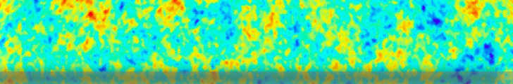
Masks

Cl classic

noise [muK arcmin]
10
10
1
1
0.1
0.1

Cl flat = 1e-17

10
10
1
1
0.1
0.1

Cl null = 0

10
10
1
1
0.1
0.1

6.2 

Comparaison effet de fsky et de masque :

• fsky = 1.0 VS fsky=0.6
• 3 types de masques : polar cap, litebird (=planck dust map), et random.
• nside=4
• nsimu = 1000
• beam =0.5 deg
• delta ell = 1 (non binning)
• r=0.1

6.3  ClEE ≠ 0

Estimateur (plots partie haut) et variance (plots partie bas), EE et BB.

Masks
\sigma=0.1 \mu Karcm
\sigma=1.0 \mu Karcm
\sigma=5.0 \mu Karcm

Histogramme Cl à ell=2 :

Masks
\sigma=0.1 \mu Karcm
\sigma=1.0 \mu Karcm
\sigma=5.0 \mu Karcm

Histogramme Cl à ell=6 :

Masks
\sigma=0.1 \mu Karcm
\sigma=1.0 \mu Karcm
\sigma=5.0 \mu Karcm

6.4  ClEE = 0

Estimateur (plots partie haut) et variance (plots partie bas), EE et BB.

Masks
\sigma=0.1 \mu Karcm
\sigma=1.0 \mu Karcm
\sigma=5.0 \mu Karcm

Histogramme Cl à ell=2 :

Masks
\sigma=0.1 \mu Karcm
\sigma=1.0 \mu Karcm
\sigma=5.0 \mu Karcm

Histogramme Cl à ell=6 :

Masks
\sigma=0.1 \mu Karcm
\sigma=1.0 \mu Karcm
\sigma=5.0 \mu Karcm

Comparaison effet de fsky et de masque :

• fsky = 1.0 VS fsky=0.6
• 3 types de masques : polar cap, litebird (=planck dust map), et random.
• nside=4
• nsimu = 1000
• beam =0.5 deg
• delta ell = 1 (non binning)
• r=0.1

6.5  ClEE ≠ 0

Estimateur (plots partie haut) et variance (plots partie bas), EE et BB.

Masks
\sigma=0.1 \mu Karcm
\sigma=1.0 \mu Karcm
\sigma=5.0 \mu Karcm

Histogramme Cl à ell=2 :

Masks
\sigma=0.1 \mu Karcm
\sigma=1.0 \mu Karcm
\sigma=5.0 \mu Karcm

Histogramme Cl à ell=6 :

Masks
\sigma=0.1 \mu Karcm
\sigma=1.0 \mu Karcm
\sigma=5.0 \mu Karcm

6.6  ClEE = 0

Estimateur (plots partie haut) et variance (plots partie bas), EE et BB.

Masks
\sigma=0.1 \mu Karcm
\sigma=1.0 \mu Karcm
\sigma=5.0 \mu Karcm

Histogramme Cl à ell=2 :

Masks
\sigma=0.1 \mu Karcm
\sigma=1.0 \mu Karcm
\sigma=5.0 \mu Karcm

Histogramme Cl à ell=6 :

Masks
\sigma=0.1 \mu Karcm
\sigma=1.0 \mu Karcm
\sigma=5.0 \mu Karcm