HPR for Monte-Carlo
Characteristics of the data:
Data simulated @ CC
| group/runname | simupapier6 |
| bolo | 143-5 |
| nSide | 512 |
| IMO | '1127593' |
| signal name | 'cmb_gal_dipcosmo_gauss' |
| first ring | 580 |
| last ring | 13080 |
In all these simulations, for the OOF Noise. Fmin is set to 1e-5 Hz. It corresponds to a period of ~1 day.
date:18/09/09
Comparison of the Different methods to substract Offsets
(N.B: All the results of the MC studied were presented in the LAL Group Meeting dated 17/09/09)
CONCLUSION:
- It seems that the limit value of fknee is around 1e-2 Hz. It is close to the expected value which is around 3e-2 Hz.
So these parameters mean that the configuration is at the limit of the Destripping Hypothesis.
Effect of the Offset Substracting Method on WN results.
Reminder about the two methods to substract offset:
The first method applied to work out the bias for WN was the 'Null' method (see below post on 31/07/09). This method consist in doesn't substracting any offset on WN HPR because there is no need to. With WN noise, there is a no long term drift so no need to substract any offset.
For a high fknee, the long term drift change the average value of the noise which is what we call the offset so it must be substracted.
Nevertheless, for fknee=1e-4Hz, it is almost the same case than WN (the long term drift is very very small). But, in order to be consistent with OOf noise with high fknee, the same method is applied to substract offset. The method to substract offset can be 'Avg' or 'ROIoffset'.
- The method 'ROIoffset' uses the offset worked out from Polkapix.
- The method 'Avg' works out the offset of the HPRnoise over the considered ring.
To explain the 'Avg' method see the graph and explaination below.
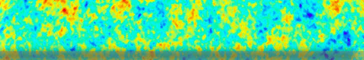
Hereafter is plotted HPRs: HPR of Signal, HPR of Signal+Noise, and the difference of the two (HPR of noise alone)
As said at the top of that page in the Data characteristics, in the HPRSignal there is cmb + galaxy + dipole cosmo.
On the HPRSignal+Noise, the noise correspond to a simulation where fknee=1e-1Hz.
It is the ring 590. Ths ring has been chosen because the offset is important. It is easy to see that because the HPRSig+Noise is quite importantly shifted down compared to the HPRSignal.
In green, the HPRnoise is plotted.
The offset obtained with the 'Avg' method is just the mean value of the HPRnoise. Here it is ~ 1.75e-3.
Effect of the Offset Substracting Method on WN and fknee=1e-4Hz results.
| Offset Method | 'Null' Method | 'Avg' Method | 'ROIoffset' Method |
| WN |
| WN |  |  |  |
| WN: mean | 1.71e-09 | 1.26e-07 | 5.41e-07 |
| WN: dispersion | 2.e-07 | 2.e-07 | 2.e-07 |
| Fknee=1e-4 |
| Fknee=1e-4 |  |  |  |
| Fknee=1e-4: mean | 6.51e-07 | 1.26e-07 | 5.41e-07 |
| Fknee=1e-4: dispersion | 2.1e-07 | 2.e-07 | 2.e-07 |
| Fknee=1e-3 |
| Fknee=1e-3: mean | 6.3e-05 | 1.34e-07 | 5.54e-07 |
| Fknee=1e-3: dispersion | 5.e-06 | 2.e-07 | 2.e-07 |
Comment:
- The first thing to note is that for the White Noise, the mean value of the histogram goes from 1.71e-09 with the 'Null' method to 1.26e-07 with the 'Avg' method. This value is then closer to the results of the fknee=1e-4 case with 'Avg' method. (see: New plot Bias_vs_Fknee with the 'Avg' method below)
- One can see that there is a significant difference between the results of the 'Avg' and 'ROIoffset' methods (~ 2-sigma). This is just because the methods estimating the offsets are different. Polkapix gives a wider dispersion of the estimated offsets. (More to be done on that).
- An important point is that for each method ('Avg' and 'ROIoffset'), the results of WN and fknee=1e-4 are very close. It means that the case fknee=1e-4Hz is actually very close to the case WN. Nevertheless, the slight difference between the two cases is pointed out by the 'Null' method. The natural dispersion of fknee=1e-4Hz is around 6.5e-07 (almost zero for WN as expected), so, of the order of magnitude of the difference of results between the 'Avg' method and the 'ROIoffset' method. It means that the extra-dispersion due to long-term drift for fknee=1e-4Hz is very very small. The case fknee=1e-3Hz has been added to show that in that case, the extra-dispersion is not negligeable anymore (results of 'Null' method) but the methods 'Avg' or 'ROIoffset' gives consistent bias.
New plot Bias_vs_Fknee with the 'Avg' method
| Bias vs Fknee | Relative Bias vs Fknee | Error vs Fknee |
 |  |  |
Comment:
- Again, the abscisse fknee = 1e-5Hz correspond to the White Noise case. On that plot, one can clearly see the change of behaviour. The left part is now flat.
- On the second plot, a relative bias of 1/1000 correspond to fknee=1e-2 Hz. It is close to fspin = 1.6e-2 Hz.
Order of Magnitude for WN:
The results obtained for the WN can be explained.
It goes from 1.71e-09 with 'Null'-method to 1.26e-07 with 'Avg'-method for the mean of the bias. And the standard deviation is 2e-7 in the two cases.
So, for 'Null' method, the mean is very close to zero (the expected value). This order of magnitude is consistent. Indeed one simulation corresponds to the cumul of 2000 rings and each ring have ~4200 bins. So one simu corresponds to ~8.4e6 samples, and then the dispersion on the mean is sigma0/sqrt(#sample) = 8.135e-4/sqrt(8.4e6) ~ 2.8e-7.
The mean value 1.71e-09 with 'Null'-method corresponds to the cumul of 4000 simulations, then #sample ~ 4000*2000*4200 = 3.36e10 and then the error on the mean is ~ 8.135e-4/sqrt(3.36e10) = 4.4e-9. This is the same order of magnitude.
For the 'Avg' method:
Let's say that the HPR unweighted noise is {xi} which is a Pur WN. For each ring, the mean is worked out: <xi>1ring = <xi>4200 because there is roughly 4200 bins per ring.
And so the new random variable is not anymore {xi} but {yi} where yi = xi - <xi>4200.
There statistics are:
{xi} -----> N0,sigma0
{<xi>4200} -----> N0,sigma0/sqrt(4200)
{yi} -----> N0,sigma0*sqrt(1+1/4200)
So, the standard deviation of {yi} is sigma0*sqrt(1+1/4200) ~ sigma0*(1+1/8400) (DL) and then the bias is sigma0/8400 ~ 1e-07 which is the right order of magnitude: 1.26e-07 with 'Avg'-method
date:31/07/09
Dispersion of the Convergence of the HPR of OOF Noise: (for the different Fknee)
CONCLUSION:
A change of behaviour around fknee~5e-3Hz is observable.
More study has to be carried to understand the effect of the method substracting the offset.
Data caracteristics:
- Histograms based on 4000 simus
 - cumulating 2000 rings
 - obtained with the 'Average' method for Oof noises and the 'Null' method for WN
| Fknee (Hz) | WN | 1e-4 | 1e-3 | 3e-3 | 1e-2 | 2e-2 | 3e-2 | 5e-2 | 1e-1 |
| Histogram | | |  |  |  |  |  |  |  |
| Residue |  |  |  |  |  |  |  |  |  |
| Mean | 1.7103950e-09 | 1.2643145e-07 | 1.3381912e-07 | 1.9323482e-07 | 8.6794673e-07 | 3.0876281e-06 | 6.7733881e-06 | 1.8457395e-05 | 7.1168136e-05 |
| Sigma | 1.9977830e-07 | 2.0010491e-07 | 2.0011942e-07 | 2.0014542e-07 | 2.0115284e-07 | 2.1672393e-07 | 2.7478727e-07 | 5.5657090e-07 | 1.9710181e-06 |
Then, with these values one can plot the bias vs fknee.
| Bias vs Fknee | Error vs Fknee |
 |  |
Comment:
- Note that the data corresponding to the abscisse fknee = 1e-5Hz are actually the data for the White Noise that should be at -infinity.
- One can see that there is a shift between WN (at fknee=1e-5) and fknee=1e-4. That artefact is due to the method used to substract the offset in HPR. For the WN, no offset is substracted because there is no offset. For fknee=1e-4 or more, the offset substracted is the one obtained with the 'Avg' method. The offset substracted is the mean of the HPRnoise ocer one ring.
- If one forgots that shift, one can easily see the change of behaviour around fknee=5e-3 Hz.
date:29/07/09
Dispersion of the Convergence of the HPR of White Noise:
As the difference of behaviour between a simulation of White Noise and Fknee=1e-2 is very close, the estimation in the case of WN should be better caracterised.
It has been seen below that even with the estimator of sigma based on the variance routine of IDL a bias still remains. Actually, it depends on the ring (for checkHPR_3) or the simulation (for checkHPR_4) considered.
Then the dispersion of this bias will be studied.
For example, for checkHPR_3, the value of the bias (the difference between the estimated and the expected value for sigma) when it has converged (so the estimation is based on accumulating a lot of simulations) will be plotted for different rings. This will be done in the new routine checkHPR_13.pro and checkHPR_13_pro.pro.
This is the same thing for checkHPR_4: the bias for different simulation is plot. (This time, the bias is evaluated with accumulating rings). It is routine checkHPR_14.pro and checkHPR_14_pro.pro.
CONCLUSION:
The remaining bias of the estimator has been understood. It is due to the intrinsic statistics of this estimator! This is the intrinsic dispersion of our estimator. Then for each value of Fknee for the OOf noise, this dispersion will be estimated as for the White Noise. These values are the error on the bias!!
A qualitative approach of the dispersion:
For the plots below:
- checkHPR_13: Few rings and ~2000 simus accumulated.
- checkHPR_14: Few simus and ~2000 rings accumulated.
- The x-axis corresponds to the last iterations of the convergence. (So it corresponds to the right part of plot: checkHPR_4 - WN, below in the post dated 23/07/09: HPR of OOF Noise and comparison with White Noise)
| checkHPR_13 | checkHPR_14 |
 |  |
Comment:
- The dispersion is roughly the same for the two cases. It is around ~3-4e-7!
- It seems to be centered around zero. So no bias in average!!
- As the the dispersion is the same for the two routines, it means that an "ergodic" hypothesis is correct !
A better estimation of the dispersion will be done on the more simulation (~5000 simus) with checkHPR_14.
A more quantitative approach of the dispersion:
Here, with checkHPR_14, 5000 simus are used and always accumulating ~2000rings.
| Convergence for differents simulations | Histogram | Residu |
 |  |  |
It gives: sigma of this distribution ~ 2.00e-7 +/- 5e-9
Comment:
- It clearly appears that the bias is centered. So, if the ring and the simulations were averaged together, there wouldn't be any bias!!
- It has a gaussian shape of sigma = 2.00e-7 +/- 5e-9.
- The residue has the amplitude of the expected poissonian error.
The reason of this behaviour can be explained !!
- Bias due to the estimator:
The first possible reason for the estimator's bias was that the estimator based on the variance routine of IDL wasn't correct. It was correct in the toy model but maybe this estimator isn't the best one. Indeed, this estimator considers that the average value of the random variable is unknown.
Then its expression is: var1 = 1/(n-1) * sum( (xi - <xi>)^2 )
But, as the average value is known: it is zero. The estimator should be: var2 = 1/n * sum( xi ^2)
So, the relation between the two estimator is: var2 = <xi> ^2 + var1 - 1/n * var1
Here, {Xi}i are the value of the unweighted noise of the HPR! And then, n is the total number of HPR bin accumulated.
What is plot everytime, is the bias; which means the difference between the estimated sigma and the expected sigma: d = sigestim - sigexpected.
So, what need to be compared is the bias with the first and the second estimator to see if the second one is better:
d1 = sig1 - sigexpected = sqrt(var1) - sigexpected and d2 = sig2 - sigexpected = sqrt(var2) - sigexpected
And the difference between the two bias is : d = d2 - d1
After the calculation, it gives: d = sig1 * ( sqrt{ 1 - 1/n + (<xi>/sig1)^2 } - 1 ).
Order of Magnitude:
- sig1 ~ sigexpected ~ 8e-4
- <xi> ~ 5e-7 (results of simulations)
- n ~ 4200*nb_of_ring_accumulated. The number of ring accumulated goes from 1 to 2000. SO for 1000 ring, it gives n ~ 4e6
An approximation can be done in the expression of d (linear development: sqrt(1+u) - 1 ~ u/2 if u << 1): d ~ sig1/2 * ( (<xi>/sig1)^2 - 1/n )
So, in term of Order of Magnitude: d ~ 4e-4 * ( (5e-7/8e-4)^2 - 1/1e6) ~ 1e-10.
Thus d ~ 1e-10 << d1 or d2 ~ 1e-6 and so the difference between the two estimators var1 and var2 should be negligeable. (That is normal because n is very big and <xi> is very close to zero !)
This results is confirmed by this plot: (don't give attention to the title or the legend. This is not the mean but the value d=d2-d1).
Comment:
- This is the good order of magnitude
- The sign is as expected: negative for few number of ring cumulated because in that case: |1/n| >> |(<xi>/sig1)^2 |
Indeed, for 300rings accumulated: n~1e6 and <xi>~1e-7!
Then the conclusion is that the bias is not due to the estimator and that the estimator is correct. (At least, sig1 gives the same results than sig2 which is the correct estimator!)
- The intrinsic statistic properties of this estimator.
The good question to ask is what is the statistic of the variance estimator: var1 = 1/(n-1) * sum( (xi - <xi>)^2 )
We will suppose that it is the same than var2 = 1/n * sum( xi ^2). And this estimator should follow a chi_square law because it is the sum of the square of gaussian random variables!
Actually, this is the following random variable that should follow the chi square law: K = var2 * n / (sigexpected ^2)
It should follow a chi square law with n degree of freedom!
This hypothesis is going to be tested:
The 'A more quantitative approach of the dispersion' section uses 5000 differents realisations of the variance var1 (or var2, these two estimator are suppose to be equivalent).
So the statistics of the random variable K can be tested:
K = var1 * n / (sigexpected ^2) = n * (sig1 / sigexpected)^2 = n * ((sigexpected + d1) / sigexpected )^2 = n * ( 1 + d1 / sigexpected )^2 = n * ( 1 + 2*d1 / sigexpected + (d1 / sigexpected)^2 ) where d1 is the bias!
Hereafter is the statistics of K:
The data used are the one used for plotting the histogram in the section 'A more quantitative approach of the dispersion'. There is 5000 different realisation. Remind that the ith elt of this 5000 elements array is the bias worked out by averaging 2000 rings (from ring 1000 to 2999) of the ith simulation.
In that case, the accumulation of 2000 ring of the HPR corresponds to 8440783 bins accumulated to workout the sigma and the the bias. This number is important here because it is the number of degree of freedom of the chi square law. So the histogram below should be centered around this value and its variance should be two time this number. (This is the caracteristics of a chi square law!)
A last remark is that the chi square law should be close to a gaussian because the number of DoF is big here!
| Histogram of Chi2 | Histogram of Proba of Chi2 value |
 |  |
And the fits gives:
mean = 8440794.8
variance = 17023254.
sigma = 4125.9246
prob_cum = 0.13477729 (this is caracteristic value based on the test to know if the data follow a chi square law. This value tell that it is OK! (The limit value is 0.1, under this value, the model is questionable))
Comment:
- First, the shape of the histogram of chi square is guassian!
- The shape of the second histogram should be a uniform histogram: the shape isn't bad but the dispersion is quite important! It is due to the fact that there is only 5000 elts used. It is too few!
- Exploitation of the values:
--- For the mean: the expected value is nb_DoF = 8440783. mean = 8440794.8, the difference ~ 11 is very small! That confirms the hypothesis of a chi square law.
--- For the variance: the expected value is 2*nb_DoF = 16881566, while the estimated value is variance = 17023254. So the difference is 141687.82 which gives a relative difference of less than 1%. Same thing, that confirms the hypothesis of a chi square law.
So, the dispersion of the bias of the convergence is intrinsic to the estimator used.
The dispersion of the random variable K, linked to the dispersion of the estimator var1 (itself linked to the dispersion of the bias), has been understood.
Then, one should be able to explain the order of magnitude of the dispersion on the bias (~2e-7 see this plot in the section: 'A more quantitative approach of the dispersion') with the caracteristics of the random variable K and the chi square law:
To link the dispersion on the bias and the dispersion on K, one have to write the relation between the two random variable (it was written above: K = n * ( 1 + 2*d1 / sigexpected + (d1 / sigexpected)^2 )
The third term can be considered as negligeable because : d1 / sigexpected ~ 1e-3 << 1 (see Order Of Magnitude above).
Then: K ~ n + n * 2*d1 / sigexpected
As expected, the mean value of K is n, the number of degree of freedom. And in this approximation, the standard deviation of K and d1 are proportionnal:
stddev of K = stddev of d1 * 2*n/sigexpected
As K follow the chi square law with n DoF, stddev of K = sqrt(2*n), then stddev of d1 = sigexpected / sqrt(2*n).
stddev of d1 ~ 8e-4 / sqrt(2*8.44e6) = 1.94717e-07 ~ 2e-7 which is the value obtained in fitting the bias of convergence! OK!!
date:23/07/09
HPR of OOF Noise and comparison with White Noise:
Now, mainly the differences of the estimated sigma with the expected sigma will be studied.
| IDL routine | checkHPR_1 | checkHPR_2 | checkHPR_3 | checkHPR_4 |
| Data caracteristics | It corresponds to the simulation 1, x-axis: between ring 1000 and 2999 | It corresponds to the ring 1000, x-axis: between simu 1 and 2000 | It corresponds to the ring 1000, x-axis: accumulate simu between 1 and 2000 | It corresponds to the simulation 1, x-axis: accumulate ring between 1000 and 2999 |
| FKnee = 1e-1 |  |  |  |  |
| FKnee = 3e-2 |  |  |  |  |
| FKnee = 1e-2 |  |  |  |  |
| FKnee = 1e-3 |  |  |  |  |
| White Noise |  |  |  |  |
Comment:
- The results for Fknee=1e-1 are clearly different from Fknee=1e-2 and the White Noise.
- Nevertheless, the results for Fknee=1e-2 (or Fknee=1e-3) and the White Noise are very close.
- The results for Fknee=3e-2 are intermediary between Fknee=1e-1 and Fknee=1e-2! OK!
date:20/07/09
HPR of White Noise (only):
This time the estimator is based on the IDL routine: variance (with the '/double' argument for numerical precision (see Estimator Behaviour)).
CONCLUSION:
This estimator still have a bias. Origin unknown for now !!!
Even with the maximum of data, the convergence isn't reached. Then for now, only ~2000 ring or simulations will be accumulate because otherwise with more data, the routines would take too much time to finish!
This remaining bias may not be a problem if the results obtained for the OOF Noise are very differents from the White Noise. (see above)
| checkHPR_1.pro : One Simu and Several Ring |
| simu = 1 | simu=1437 |
| Sigma | Difference with expected value | Sigma | Difference with expected value |
 | |  |  |
| checkHPR_2.pro : One ring and Several Simu |
| ring=1000 | ring=3000 |
| Sigma | Difference with expected value | Sigma | Difference with expected value |
 | |  |  |
| checkHPR_3.pro : One ring and Accumulate Simu |
| ring=1000 | ring=3000 |
| Sigma | Difference with expected value | Sigma | Difference with expected value |
 | |  ? ? |  |
| checkHPR_4.pro : One Simu and Accumulate Ring |
| simu = 1 | simu=1437 |
| Sigma | Difference with expected value | Sigma | Difference with expected value |
 | |  |  |
Comment:
- For checkHPR_1 and 2, the bias has disappeared. For checkHPR_3 and 4, a bias still exist. The convergence might not be reached yet or this estimator isn't good enough too.
- To check if the convergence hasn't been reached yet, see right below.
Study the convergence further:
It will be only studied with checkHPR_4 (actually the plots below were obtained with checkHPR_4bis.pro a checkHPR_4.pro-modified routine that allow to study the convergence with a lot more ring accumulated.)
On the plots below, almost all the rings of the survey have been included for the right part of plots. It corresponds to ~ 12000 rings accumulated.
| For simu = 1 | For simu = 2538 (this noise realisation is particularly biased) |
 |  |
Comment:
- In the two case, it doesn't converge.
- For simu=2538, the bias moves closer and closer to 0 but doesn't reach it.
- For simu=1, the bias is very close to 0 and then move away from it slowly.
It clearly appears that the convergence isn't reached even with the maximum of data available. We will have to deal with it and then, generally, the number of ring (or simulation) used for estimating the bias will be ~2000 in order to have an acceptable running-time of routines.
date:16/06/09
HPR of White Noise:
The first thing is to do is to check that we have the correct sigma_sample by fitting the HPR of noise (unweighted by the HPR of Hit).
The expected value for sigma_sample is 8.13548e-4
The estimator of sigma used is the following one:
An histogram of the noise is made and the estimator is the sigma value given by the gaussfit routine of IDL.
CONCLUSION:
The first results show that the estimator chosen is biased (see below and Estimator Behaviour).
The post above is using an other estimator (the simple IDL variance).
One ring and One simu:
ring=1000 and simu=1
| HPRs | HPR of Pure Noise ( with weight) | HPR of Pure Noise (unweighted) | Histogram of Unweighted HPR and Fit |
 |  |  |  |
| - FIT RESULTS - |
| Reduced chi2 | 0.88254949 |
| Number of DOF | 4224 |
| sigma_estimated | 0.00080888311 |
| sigma_sample | 0.000813548 |
| Err on Sigma_Estim | 9.4239585e-06 |
| Relative Deviation | -0.0057336331 |
| nb_of_sigma | -0.49497077 |
Comment:
The results is consistent with the Expected value (the results is at 0.5-sigma for the first case).
But this results depends on the ring and the noise simulation chosen. And as the number of sample used for the fit is small (~ 4000 (number of Degree of Freedom)), the error might be important.
So the same study will be done on several rings and several noise simulations to be sure that the same results is obtained.
One simu and several ring accumulated together:
simu=1 and from ring 1000 to 3999 (3000 rings)
| HPRs | HPR of hit |
 |  |
| HPR of Pure Noise (with weight) | Histogram of HPR and Fit | Residue and Error |
 |  |  |
| HPR of Pure Noise (unweighted) | Histogram of Unweighted HPR and Fit | Residue and Error |
 |  |  |
| - FIT RESULTS - |
| Reduced chi2 | 0.921228 |
| Number of DOF | 12674107 |
| sigma_estimated | 8.13503e-4 |
| sigma_sample | 8.13548e-4 |
| Err on Sigma_Estim | 1.61551e-07 |
| Relative Deviation | -5.55212e-05 |
| nb_of_sigma | -0.279596 |
Comment:
The results is very good with a relative deviation from the expected sigma of -5e-5.
This results still depends on the noise simulation chosen.
One ring and several simu: (checkHPR_2.pro)
| ring = 1000 and simu between [1,2000] |
| Estimed Sigma | Error on Estim Sigma | Difference | Nb of Sigma |
 |  |  |  |
| ring = 3000 and simu between [1,2000] |
 |  |  |  |
One simu and several ring: (checkHPR_1.pro)
| ring between [1000,2999] and simu=1 |
| Estimed Sigma | Error on Estim Sigma | Difference | Nb of Sigma |
 |  |  |  |
| ring between [1000,2999] and simu=1437 |
 |  |  |  |
Comment:
- Sigma seems to be under-estimated compared to the expected value in every case!! (Even if 0 is between one and two sigma of the distribution).
- One can see that the dispersion on sigma and the estimated error on sigma are consistent (around 1e-5)
More check: An other check is to accumulate the HPRnoise for different ring or simulation and do a common fit. Because the bias may be due to too few elements in the HPR. (see below)
ACCUMULATE of several simu and One ring: (checkHPR_3.pro)
| ring = 1000 and simu between [1,2000] |
| Estimed Sigma | Error on Estim Sigma | Difference | Nb of Sigma |
 |  |  |  |
| ring = 3000 and simu between [1,2000] |
 |  |  |  |
ACCUMULATE of several Ring and One Simu: (checkHPR_4.pro)
| ring between [1000,2999] and simu=1 |
| Estimed Sigma | Error on Estim Sigma | Difference | Nb of Sigma |
 |  |  |  |
| ring between [1000,2999] and simu=1437 |
 |  |  |  |
Comment:
- The fitted value converges but, it is not always toward the expected value. The estimation seems still biased.
- Nevertheless, the relative deviation to the expected value is very small: around 1e-3
The reason of this bias might be linked to the sigma estimator.
It seems that there is a constant bias with this estimator. To evaluate this effect, the estimator's behaviour is tested here: Estimator Behaviour.